Data Science Tropes: Cowboys and Sirens
As Abraham Maslow—he of the eponymous hierarchy of needs—said in 1966, “I suppose it is tempting, if the only tool you have is a hammer, to treat everything as if it were a nail.” To a fledgling Data Scientist (say, a college sophomore) who has just found out about the wonders of Machine Learning (ML), nothing beats the adrenaline rush of discovering their hammer: the ability to sign up on Kaggle, install xgboost, fire up a Jupyter notebook and, within 10 minutes, submit their first Machine Learning model in a competition. As it happens, xgboost is the hammer of choice for most Data Science cowboys, a distinct subset of the scientific community that has appropriate Data Science training, but typically disregards or doesn’t understand the correct way to handle ML and Artificial Intelligence (AI) technology.
Xgboost is the perfect, yet risk-fraught, hammer for these cowboys because it demands little data pre-processing, including scaling and normalizing data, and doesn’t carry out missing value imputation. Even if xgboost had them, these qualities would be lost on the Data Science cowboy, who likely would not have an understanding of the 35 parameters that influence the nature of the model because she or he primarily relies on default parameter values, anyway.
The Handle of the Hammer: Decision Trees
Decision trees have been around for quite a while and have been used in a variety of scenarios, especially when model transparency is required. Tree structures can perform better than logistic regression and scorecards when the amount of data available is not large and few variables are present. But data scientists share a common understanding that the decision tree construct is prone to instability in the presence of noise, and often drifts toward overfitting due to its tendency to slice and dice the data ad infinitum.
Decision trees locate hard boundaries inside the input features and give discontinuous predicted outcomes across the boundaries. This is occasionally a virtue—if the phenomenon is robust enough to deserve a hard call-out—but more often a vice, if the so-induced decision boundaries home in on unusual fluctuations and peculiar combinations of feature values which don’t have a real-world justification.
Read more: The History and Future of Data Science
Decision trees don’t make smooth outcome surfaces, and more unsettling, they don’t bound gradients of the predicted outcome with respect to input variables. This is due to a lack of algorithmically guided error reduction, in which the error is attributed proportionally to the partial derivates of the input variables.
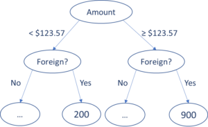
The consequence? Infinitesimal differences in the input variables may lead to disproportionately large differences in the score. Figure 1 shows an example of a decision tree where such large and unbounded gradients lead to unstable and unreasonable score behavior as the transaction amount increases from $123.56 to $123.57.

Fig. 1. A partial view of a data-driven decision tree that segments on amount followed by whether it is a foreign or a domestic transaction. For a $123.57 foreign transaction, we observe a change of 700 points in the score for a one-cent change from $123.56, an output variance that is wildly disproportionate to the one-penny difference in inputs. This does not meet standards of model palatability, which leads to such models being rejected by model governance.
In this figure, the leaf nodes are the scores generated by the model, as inferred from the training examples residing in those leaf nodes. In this decision tree, $123.56 foreign transaction is scored at a risk level of 200, while a $123.57 foreign transaction sends the score soaring 700 points to 900. For a one-penny difference in amount, the gradient is then 70,000 score points/dollar, an output variance that is wildly disproportionate to 1¢ difference in inputs. This example vividly illustrates that with the data science—and business—world’s increasing emphasis on the explainability, reliability, and consistency of models used for decisioning, decision trees simply lose a lot of their palatability.
In contrast, smooth models such as logistic regression and neural networks are continuous in their input variables, and common regularization methods (i.e., ridge and lasso regression) limit their sensitivity to inputs. Newer regularization principles from deep learning literature, such as singular value constraints, and training techniques (i.e., batch normalization and numerous others) inhibit large input-output gradients even in complex multi-layer neural networks.
Turning back to decision trees, the regularization methods in this software are even more heuristic and less justified than for neural networks—and there’s no control over input sensitivity.
Decision Trees Amplify Small Anomalies
Experienced data science practitioners accept the truism that models are more overfitted than they appear. One key reason is that inevitably, there is more correlation between real-world input examples than assumed by train-and-test randomization procedures. This makes the usual “out” of sample evaluations still too optimistic.
Consider a burst of fraud examples that arose from a single fraud ring with a common modus operandi and geographic period. These examples might not all be linked and identified in the training set, so a typically randomized hold-out set will contain some examples of this fraud ring in both train and test data sets. Supervised decision trees sniff out a peculiarly anomalous and small piece of input space that’s discontinuous from neighbors, and amplify this effect.
How to ameliorate this over-sensitivity? Use smoother models, ensure that discontinuous splits of space are constructed or reviewed by humans with real-world experience with the phenomenon, and ensure that global constraints like monotonicity are in place.
Gradient Boosting Amplifies Model Risk
Boosting, particularly gradient boosting, of large tree ensembles amplifies the inherent risks of decision trees. The idea of gradient boosted decision trees (GBDT) is to train a succession of decision trees; this starts with the first tree to fit on the given data, and the second tree of the residual produced by the first one, and so on. Each residual procedure further increases noise and exacerbates the tendency of decision trees to isolate small parts of input spaces and increases substantially the sensitivity to noise. This is how overtraining occurs.
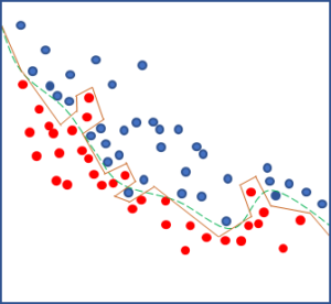
The internal randomization procedures of GBDT, implemented in software libraries like xgboost, nearly always assume independence of input samples, increasing the risk of overfitting. There is no control over smoothness, and the advantage of single decision trees, human interpretability, is abandoned in the large ensemble of trees trained on different datasets. Figure 2 shows a two-dimensional projection of an overfitted decision boundary separating the red and blue classes generated by a GBDT model (orange) and contrasted with the smooth and robust decision boundary (green) generated by alternative algorithms.

Fig. 2. A two-dimensional projection shows the choppy and unstable overfitted decision boundary generated by a GBDT model (orange) compared with the smooth and robust decision boundary generated by an alternative algorithm (green).
Combined with the tendency of both decision tree and boosting to produce overfitting, we end up with a choppy and unstable decision boundary that reflects the well-learned data and noise. Heuristic pruning and trimming fails to effectively address this deficiency because there is insufficient mathematical guidance on where to focus efforts. As a result, there is no safe way to control input sensitivity or discontinuities or compensate for the excess correlation between training examples versus a real-world out-of-time application.

GBDT tempts data scientists—to their detriment
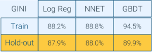
With results too good to be believed, GBDT becomes the Homeric siren calling to the data scientist who has set sail on choppy data seas. One such performance result is shown in Figure 3. The significant drop in the performance of the GBDT model convincingly indicates that the model is over-trained, and as such should not be deployed. Still, the GBDT siren would beckon to the data scientist with the much larger training performance result. However, the size of model performance drop on the hold-out dataset, as compared to the model performance on the training dataset, foretells the story of the ship heading straight for the rocks.
Why? Because the over-trained model has learned the noise of the data, not some hidden non-linear relationship. The seemingly high -performance number on the holdout dataset has very low confidence associated with it. Furthermore, the fact that the neural network, which is capable of learning significant feature combination and nonlinearity, performs similarly to logistic regression (Log Reg) shows that the major non-linearities have already been captured by the feature engineering which produced the input variable set.
Simply put, the GBDT is fitting to random fluctuations in small pockets of the input space, which should not be trusted to be robust in a practical deployment out of time.
Inexplicable Behavior
Both the logistic regression and neural network models show a well-generalized performance scenario on in-time and out-of-time data. Deeper inspection shows that the GBDT model further produces significant undesirable behavior where the output score was distinctly non-monotonic, and trending in the wrong direction over large regions and multiple variables. This behavior is not explainable or justifiable to a human regulator or customer and is likely to be mispredictive in future situations.
The bottom line: We can control monotonicity in logistic regression, neural networks, and generalized linear models with known technology, but not with tree ensembles. Monotonicity is a fundamental requirement for sensible models, and the lack of ability to control it in GBDT is of considerable concern.

Fig 3. Comparative model performance on training and holdout datasets: The performance of logistic regression (Log Reg) and neural network (NNET) models remain similar across the training and the hold-out datasets showing proper generalization of true fundamental drivers of the model score. But applying GBDT shows a large performance difference between the training and the hold-out datasets, thereby demonstrating non-real relationships and noise learned on the training set which do not generalize to the hold-out set.
The Lyrics of the Siren’s Song
The heuristic behind GBDT can provide a seemingly powerful model with minimal effort on the data handling part, without the need to adjust any of the multitude of knobs and levers that control the model training. This seeming ease, accompanied by the tendency of a GBDT model to easily overfit (particularly in ways that are not visible in the usual cross-validated hold out methodology implemented in software), increases the risk of a machine learning model shipwreck while sailing on the rough ocean of deployed production use.
Why do GBDT hammers seem to be behind the winning entries in Kaggle contests? First, a contest’s test-sets are never as different as in real life out-of-time behavior. Second, the vice of GBDTs––amplifying noise––can be a virtue. The criteria to win on Kaggle are skewed to place among the very top results; when there are many nearly equivalent competitive entries, a noisy model might be sufficiently fortuitous to match the contest’s hold-out set in particular examples. To win Kaggle, it’s better to be risky and lucky than to be safe.
Don’t Be a Trope
To sum it all up with a mishmash of metaphors, don’t be a data science cowboy with an xgboost hammer who becomes mesmerized by the siren song of gradient boosting. In practical applications with impactful consequences, we need reliable, explainable models with well-defined, smooth and stable scores that generalize well on yet-unseen data, such as the aforementioned neural network model. Although there is a place for tree ensembles in data exploration and insights for feature engineering (Random Forests to GBDTs are preferred for this purpose), it is wiser to keep GBDT out of deployed models and instead rely on alternative techniques.
Read more: Ultimate Data Science Projects to Boost Your Knowledge and Skills

Comments are closed, but trackbacks and pingbacks are open.